Dear friends,
In operations management, the lens of forecasting provides a clear path through the often foggy future of organizational planning and decision-making. This article takes you through an in-depth exploration of various forecasting methods, highlighting their applicability and impact on operations. Are you ready? Let’s go! 🚀
Why Forecasting in Operations Management?
Forecasting stands as a systematic effort to anticipate future events based on the patterns and information available from past data. Within the domain of operations management, forecasting takes a significant role, acting as an aiding tool for decision-making, strategic planning, and efficient resource allocation. Proper forecasting can significantly reduce costs, optimize processes, and pave the way for better organizational performance.
Qualitative methods are primarily subjective, relying heavily on human judgment. They do not use past numerical data; instead, they depend on expert opinions, market research, and other non-quantitative information sources. These methods are particularly valuable when historical data is not available or when predicting new, unprecedented events. Quantitative methods rely on mathematical and statistical tools to derive forecasts. By examining past data, these techniques identify patterns, relationships, and trends to predict future events. Quantitative methods are best suited for situations with a substantial amount of historical data, where the objective is to extrapolate those patterns into the future.
👥Overview of Qualitative Methods
Delphi Method
Named after the ancient Oracle of Delphi, this method seeks to arrive at a consensus among a group of experts. The process is iterative: experts provide their forecasts anonymously, then a facilitator compiles and redistributes the results for another round of predictions. The method continues until a consensus emerges. The anonymity of the process helps reduce bias and the influence of dominant personalities, allowing for a more balanced outcome.
Market Research
This approach involves gathering information directly from the market, typically from potential customers. Methods such as surveys, focus groups, and interviews are commonly used. By understanding customer preferences, attitudes, and intentions, organizations can anticipate market demands or reactions to new products.
Expert Judgment
Sometimes, simple reliance on the judgment of someone with expertise in a particular area is the best approach. This expert can draw upon their knowledge, experience, and intuition to make a prediction. While valuable, this method’s accuracy can vary widely, depending on the expert’s depth of knowledge and the unpredictability of the subject matter.
Scenario Building
Rather than predicting a single outcome, scenario building involves creating multiple plausible future scenarios based on varying assumptions. These scenarios help organizations prepare for a range of possibilities and understand the implications of different future events.


📊 Overview of Quantitative Methods
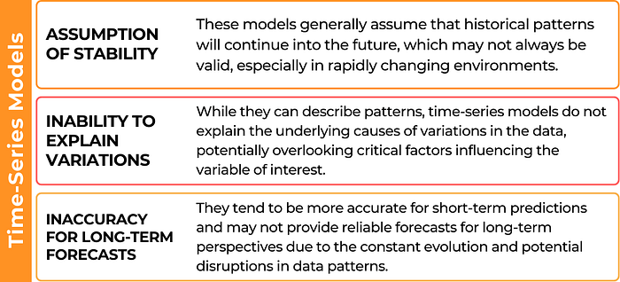
1️⃣Time-Series Analysis
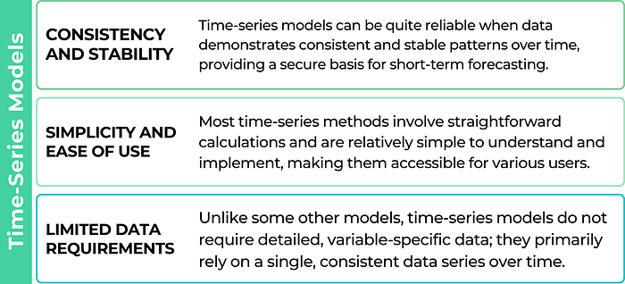
Among the various quantitative approaches, time-series analysis is one of the most widely used due to its applicability in capturing patterns over time. This section provides an insight into the core concepts and methods associated with time-series analysis.

📌Simple Moving Average (SMA)
A moving average, often referred to as a simple moving average, calculates the average of a specific number of data points taken from a dataset. It then “moves” forward by dropping the oldest data point and adding a new one, and the average is recalculated. Mathematically, for a given set of data points x1, x2,… xn, a 3-period SMA would be calculated as:
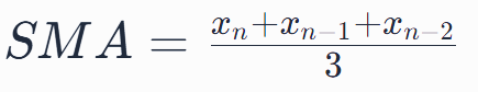
This process continues, shifting or “moving” through the dataset, which gives the method its name. The result is a smoothed line that better represents the underlying trend.
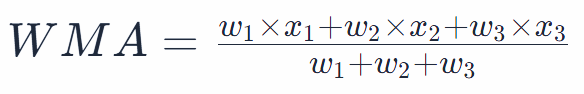
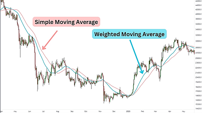
📌Weighted Moving Average (WMA)
While SMA gives equal importance to all data points in the period, sometimes it’s beneficial to weigh recent data points more heavily. The rationale is that more recent data might be more indicative of future events. In a weighted moving average, each data point in the period is multiplied by a weight, and the sum of these products is then divided by the sum of the weights. For instance, for a 3-period WMA with weights w1, w2, w3 for the data points x1, x2, x3, the WMA would be:
👣Example
Consider monthly sales data for a product: January (100), February (110), and March (90). Using a 3-month SMA, the average for March would be (100+110+90) /3 = 100. If we apply a WMA with weights of 0.5, 1, and 1.5 for January, February, and March respectively, the weighted average for March would be:
(0.5 × 100 + 1 × 110 + 1.5 × 90) / 3 = 103.33
The WMA gives a slightly higher average due to the higher weight applied to the more recent month of March.
📌Exponential Smoothing
Exponential smoothing stands out as one of the fundamental forecasting techniques in time series analysis, designed to predict future values by assigning exponentially decreasing weights to past observations. The central premise of this method is straightforward: more recent observations are typically more indicative of the future than older ones. Thus, they are assigned greater importance in predicting future values.
Mathematically, the exponential smoothing forecast is represented as:
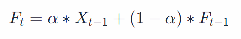
where Ft is the forecast for the current period, Xt−1 is the actual observation for the previous period, Ft−1 is the forecast for the previous period, and α is the smoothing constant (between 0 and 1).
An α value closer to 1 places more emphasis on recent observations, making the forecast more responsive to changes, while an α value closer to 0 makes the forecast more stable but less responsive.
👣Example
Let’s consider a retailer tracking weekly sales of a particular item. Suppose the sales for the previous week were 150 units, and the forecast made for that week was 140 units. If we choose a smoothing constant α=0.2, the forecast for the upcoming week would be:
Ft = 0.2 ∗ 150 + (1−0.2) ∗ 140 = 142
Thus, the retailer can anticipate selling approximately 142 units of the item in the upcoming week based on exponential smoothing.
📌Exponential Smoothing with Trend Adjustment
Exponential Smoothing with Trend Adjustment, commonly referred to as Holt’s method, refines the basic exponential smoothing technique by accounting for both the underlying level and trend in the data. This dual consideration allows for more accurate forecasting when a discernible trend is present in the time series data.
Mathematically, Holt’s method is characterized by two smoothing equations. The first equation captures the level, and the second equation captures the trend. Given yt as the observed value at time t, the equations can be defined as:

where lt is the smoothed value for period t and α is the smoothing parameter for the level.
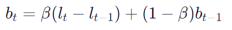
where bt is the trend factor for period t and β is the smoothing parameter for the trend.
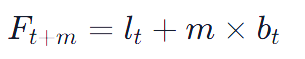
The forecast for m periods ahead, Ft+m, is then given by:
👣Example
Let’s Imagine a company that has been experiencing consistent growth in quarterly sales. Using Holt’s method, the company analyses past sales data and determines both the level and trend equations. Suppose the last observed sales data was 150 units, with a smoothed value (lt) of 145 units and a trend factor (bt) of 5. For a forecast one quarter ahead, the prediction would be:
Ft+1 = 145 + 1 ×5 = 150
Thus, the company would anticipate sales of 150 units in the next quarter.
📌ARIMA and Advanced Forecasting Models
ARIMA, standing for Auto-Regressive Integrated Moving Average, is a prominent time-series forecasting method used to analyze and predict data points in a series. The model’s strength lies in its ability to encompass different structures in data through its components:
AutoRegressive (AR) term: This captures the relationship between an observation and a specified number of lagged observations. Think of it as looking back a few steps. If you’re on the tenth step of a staircase, the AR term considers how high the eighth or ninth steps were to guess the height of the eleventh. Mathematically, the AR term can be represented as:

where yt is the observation at time t and ϕ represents the coefficient of the lagged observation.
Integrated (I) term: This represents the difference between the observations, which helps in making the series stationary (differencing). Stationarity means that the series has a consistent mean, variance, and autocorrelation structure over time.
Moving Average (MA) term: This component models the relationship between an observation and the residual error from a moving average model applied to lagged observations. Imagine averaging out errors in your past weather predictions to make today’s guess more accurate. If you’ve been off by a few degrees recently, this helps adjust today’s prediction. The MA term can be mathematically expressed as:
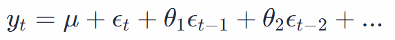
where ϵt is the white noise error term.
Beyond ARIMA, there are variants and extensions, such as Seasonal ARIMA (SARIMA) and ARIMAX, which account for seasonal patterns and exogenous variables, respectively.
For those of you who are interested, in implementing ARIMA and its variants, both R and Python are popular choices. In 🖥️R, the `forecast` package offers robust tools, while in 🖥️Python, the ‘statsmodels’ library provides comprehensive functionalities for time-series forecasting.
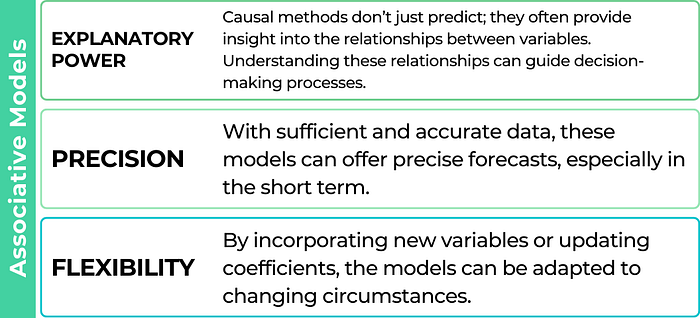
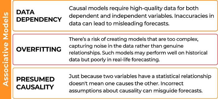
2️⃣Associative Models
Associative models, often termed causal methods, predict the future based on a presumed cause-and-effect relationship between independent (x) variables and the dependent (y) variable of interest.
📌Simple Linear Regression
Simple linear regression stands as one of the foundational methods in statistical forecasting, designed to predict the value of a dependent variable based on the value of an independent variable. The underlying principle is to establish a linear relationship between the two variables, and once this relationship is determined, future values of the dependent variable can be predicted.
Mathematically, the relationship is represented as:
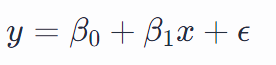
where y is the dependent variable, x is the independent variable, β0 is the y-intercept, β1 is the slope of the regression line, and ϵ represents the error term.
The goal of simple linear regression is to find the best-fitting straight line that captures the relationship between x and y. The best-fitting line is typically determined using the least squares method (OLS), which minimizes the sum of the squared differences (errors) between the observed values and the values predicted by the model.
👣Example
Suppose we want to predict the sales of a product based on its advertising budget. After gathering data and plotting it on a graph, we notice a linear trend. Applying simple linear regression, we might derive an equation like:
Sales = 50 + 5×Advertising Budget = 50 units
This equation suggests that with no advertising (a budget of $0), sales will be 50 units. Moreover, for each additional dollar spent on advertising, sales increase by 5 units.
📌Multiple Regression
Multiple regression is an extension of simple linear regression and a statistical technique used to predict the value of one dependent variable based on the values of two or more independent variables. The primary aim of multiple regression is to refine our predictions by accounting for multiple influencing factors.
Mathematically, a multiple regression model can be represented as:
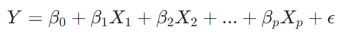
where Y is the dependent variable we are trying to predict, β0 is the y-intercept, β1, β2, … are the coefficients of the independent variables, X1, X2, …. These coefficients indicate the change in the dependent variable for a one-unit change in the independent variable while holding other variables constant, and ϵ is the error term, capturing the variability not explained by the independent variables.
The primary goal in multiple regression is to determine the best-fitting line (or hyperplane, in higher dimensions) that describes the relationship between the dependent variable and multiple independent variables.
👣Example
Imagine a retailer trying to predict monthly sales (Y) based on advertising spend (X1) and the number of salespersons (X2). Using multiple regression, the retailer might find an equation like:
Sales = 5000 + 10∗X1 + 200∗X2
This suggests that for each additional $1,000 spent on advertising, sales might increase by $10 (β1), and for each additional salesperson, sales might increase by $200 (β2), assuming the other variable remains constant. This model can then be used to predict future sales based on different scenarios of advertising spend and salesperson allocation, thereby aiding strategic planning and resource allocation.
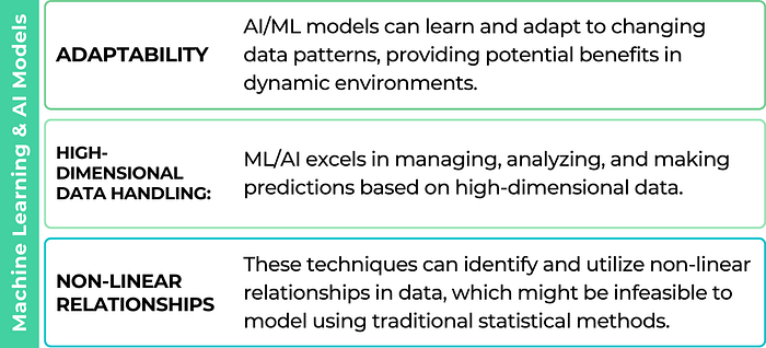
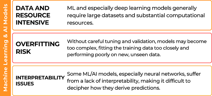
3️⃣ Machine Learning and AI Models
Machine learning and AI techniques are rapidly revolutionizing the field of forecasting in operations management. These techniques offer a number of advantages over traditional forecasting methods, such as the ability to learn from complex data patterns and to forecast nonlinear relationships. While I’m limiting this article to providing an initial overview, I encourage the curious reader to seek out scholarly articles and specialized literature for a more thorough exploration of each model’s functionality.
📌Decision Trees and Random Forests
Decision trees split data into subsets based on specific criteria. They are visual and easy to interpret, mapping out decisions and their potential outcomes. A random forest, an ensemble method, utilizes multiple decision trees to produce a more accurate and stable forecast by averaging the results.
📌Support Vector Machines (SVM)
Originally designed for classification tasks, SVMs can also be applied to regression (and thus forecasting) problems. They operate by finding the optimal boundary that separates different classes of data, and in the context of forecasting, SVMs aim to find the function that best fits the data.
📌Gradient boosting machines
Gradient boosting machines are a type of machine learning algorithm that can be used to improve the accuracy of other forecasting models. They work by iteratively adding new models to the ensemble, each of which focuses on correcting the errors of the previous models. Several variants of boosting methods exist, such as AdaBoost and XGBoost, each with its own unique approach to optimizing model performance. Furthermore, gradient boosting machines can be combined with different base learners, like decision trees or linear models, to cater to specific data characteristics. Through these methods, gradient boosting machines have been shown to achieve state-of-the-art forecasting performance on a variety of datasets.
📌Neural Networks and Deep Learning Methods
Neural networks, computational models inspired by the human brain’s structure, consist of interconnected nodes that process and transmit data. These networks come in various architectures like feedforward neural networks, convolutional neural networks (CNNs), and recurrent neural networks (RNNs). Deep learning, a subset of ML, delves deeper into these architectures, with models such as long short-term memory (LSTM) networks amplifying their potential. Both neural networks and deep learning models excel in recognizing nonlinear relationships in data, with specific designs like RNNs and LSTMs being notably effective for time series forecasting due to their ability to remember long sequences and intricate patterns.
Some specific state-of-the-art tools for machine learning and AI forecasting in operations management include:
- Facebook Prophet: A forecasting tool that uses a combination of exponential smoothing and additive regression to model time series data. Prophet is particularly well-suited for forecasting data that exhibits trends, seasonality, and holidays.
- TensorFlow Time Series (TFTS): TensorFlow, known primarily for deep learning, offers a module for time series forecasting. TFTS provides the necessary tools to work with time series data and construct forecasting models using deep learning.
- Amazon Forecast: This is a managed service provided by AWS, leveraging machine learning to deliver highly accurate forecasts. It automatically examines multiple algorithms, selects the best for your data, and requires no machine learning experience to use.
- ForecastPro: A commercial forecasting tool that offers a variety of machine learning and AI forecasting models, including deep learning, ensemble forecasting, and time-series models.
Model Evaluation and Selection
Having metrics and criteria to evaluate these models becomes fundamental to the forecasting process. Let’s discuss methods for evaluating and selecting forecasting models.
📌Forecast Error Measurement
The accuracy of forecasts is determined by measuring the difference between the forecasted values and the actual outcomes. Several metrics assist in quantifying this error:
- Mean Absolute Error (MAE): This metric calculates the average of the absolute differences between forecasted and actual values. Mathematically:

where Fi represents the forecasted value, Ai is the actual value for the ith observation, and n is the number of observations.
- Root Mean Square Error (RMSE): RMSE takes the square root of the average of squared differences between forecasted and actual values. It is given by:

- Mean Absolute Percentage Error (MAPE): This metric provides a percentage-based error, making it useful for comparisons across datasets of varying scales.

📌Bias and Variance
Bias refers to the systematic deviation of forecasts from actual values. A positive bias indicates consistent overestimation, while a negative bias denotes consistent underestimation. Ideally, an unbiased model will have errors that average out to zero. Variance, distinct from bias, emphasizes the model’s sensitivity to fluctuations in the training data. A model with high variance is likely to overfit the training data, capturing noise along with the underlying pattern. Conversely, a model with low variance might underfit, missing out on capturing the pattern altogether. In predictive modeling, achieving a balance between bias and variance becomes a central challenge. A model’s total error is composed of bias, variance, and irreducible error. To ensure the model’s generalization to new, unseen data, this balance between bias and variance must be optimized. For a deeper dive into the bias-variance tradeoff, consider referring to this article for a comprehensive exploration.
👣Example
Imagine we have forecasted demand for a product over four months, and we also have the actual demand for those months.
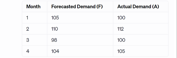
- MAE: (5+2+2+1) / 4 = 2.5. The average absolute error is 2.5 units, suggesting predictions deviate by 2.5 units on average.
- RMSE: √(5² + 2² + 2² + 1²) ≈ 2.55. An RMSE of 2.55 indicates a slightly higher penalty for larger errors, giving a more sensitive measure of forecast accuracy.
- MAPE: (5/100 + 2/112 + 2/100 + 1/105) ≈ 2.42%. A MAPE of 2.42% means that, on average, the forecasted values are off by about 2.42% from the actual values.
📌Model Selection Criteria
Beyond error metrics, selecting a forecasting model involves considering other criteria:
- Simplicity: Often, simpler models are preferable because they are easier to understand, communicate, and implement.
- Cost: The monetary and time resources required to implement and maintain the model should be considered.
- Adaptability: A model’s ability to accommodate changes or new data can be pivotal when the environment is dynamic.
Challenges of Forecasting
Forecasting, regardless of its methodological approach, grapples with a set of inherent challenges. Acknowledging these impediments is the first step towards refining our predictive capabilities. This section highlights some of the most pressing issues in the forecasting domain.
📌Data Quality Issues
Foremost among the challenges is the issue of data quality. Accurate forecasting depends on accurate data. If the historical data used to feed forecasting models is fraught with errors, inconsistencies, or missing values, the resultant predictions can be misleading. For instance, outdated information might not capture recent shifts in market dynamics. Furthermore, discrepancies between datasets, such as inconsistent units or time frames, can introduce further inaccuracies. Cleaning and preprocessing data to ensure its quality often consume a significant portion of the forecasting effort.
📌Complex Relationships
Real-world systems, especially in fields like economics, finance, and social sciences, often exhibit intricate relationships between variables. Predicting outcomes in such systems means considering interactions that might not be immediately apparent. Linear models, while simpler and more interpretable, might fall short in capturing these complexities, necessitating the use of more advanced techniques that bring their own set of challenges.
📌Structural Breaks
Structural breaks refer to sudden and significant changes in a time-series dataset. These can be due to policy changes, technological innovations, major events (like natural disasters or COVID19), or other influential factors. Such breaks can drastically alter the underlying dynamics of the data, making past patterns less relevant for future forecasting. Detecting and adjusting for these breaks is often challenging, especially when they are not anticipated.
📌Exogenous Variables
Exogenous variables are external factors that can influence the variable being forecasted but are not explicitly included in the forecasting model. Neglecting important exogenous variables can lead to biased or imprecise predictions. For instance, a model predicting a country’s GDP might miss the mark if it doesn’t factor in global economic trends or geopolitical events.
📌Resource Constraints
Forecasting often requires computational resources, especially when dealing with large datasets or sophisticated models. Resource constraints can limit the complexity of models used or the amount of data processed, potentially affecting prediction accuracy. Additionally, constraints can also be in terms of human resources. Skilled forecasters or experts in a particular field might be in short supply, limiting the depth or breadth of analysis possible.
Applications of Forecasting in Operations Management
Forecasting functions as a guiding instrument within various elements of operations management, effectively allocating efforts and resources.
📌Demand Forecasting
Forecasting demand helps businesses anticipate how much of a product or service customers will want in the future. This information can be used to make decisions about how much to produce, how many employees to hire, and how much inventory to stock. Additionally, understanding how demand fluctuates can help businesses set better pricing and promotional strategies.
📌Inventory Management
Holding too much inventory can be costly in terms of storage, potential obsolescence, and tied-up capital. On the other hand, too little inventory risks stockouts, lost sales, and potentially unhappy customers. Accurate forecasting provides a balanced view, allowing businesses to maintain optimal inventory levels, and minimize costs while ensuring product availability.
📌Production Planning
Forecasting future demand allows businesses to plan their production more effectively. This includes determining the quantity, timing, and location of production. Accurate forecasting can help businesses reduce waste, ensure on-time deliveries, and even impact sourcing decisions.
📌Scheduling
Whether it’s scheduling shifts for workers, machine maintenance, or delivery routes, forecasting plays a role. In industries where personnel needs fluctuate, such as retail or hospitality, predicting busy periods and downtimes ensures that businesses are neither understaffed nor overstaffed. Meanwhile, in manufacturing, predicting machine wear and tear can guide maintenance schedules, ensuring minimal disruption.
📌Supply Chain Management
Forecasting affects the entire supply chain, from raw material procurement to product delivery. By understanding future demands and potential bottlenecks, businesses can optimize their supply chain processes. This might involve selecting suppliers, determining order quantities, or deciding on transportation methods. A well-informed forecast can help to streamline operations and reduce lead times.
It’s evident that while perfect forecasting remains an elusive goal, the pursuit of precision holds significant weight in operations and financial outcomes. Minor deviations or misinterpretations can cascade into broader operational inefficiencies and missed opportunities. The dynamic nature of the future underscores the need for ongoing assessment and refinement of forecasts, ensuring they align with ever-evolving circumstances. Furthermore, integrating forecasting seamlessly with other core business activities, from budgeting to strategic planning, enhances its utility, helping businesses make informed and strategic decisions.